mind the gap.

Exploring Political Gerrymandering in the 2012 Federal Congressional Election

What is gerrymandering?

An ingrained facet of American democracy since the 1800’s, gerrymandering refers to the process of drawing voting district lines in a way that offers a political advantage to a specific political party or group of people. This process is a hot-button issue in the current American political climate, as experts debate whether the construction of non-competitive districts in state and federal elections has contributed to the polarization of the political landscape, while legal arguments on the lawfulness of this practice have reached the Supreme Court. The drawing of district lines determines the political representation of a state’s population, with each district sending one representative to state or federal governing bodies, and can therefore have serious societal ramifications.


District lines throughout the country are mostly redrawn every ten years, after a new census identifies the sociological makeup of a state’s residents. In most states, this line-drawing process is controlled by state legislatures. If one political party has universal control over the legislature, they could use this power to draw lines that offer them a political advantage and the possibility to earn a disproportionately high number of representative seats. Let’s look at an example of how manipulating district lines may lead to such a disproportionate advantage. Below we explore a couple district border-drawing scenarios in an example state, which has an equal number of votes between a Red and Blue political party. In each scenario, we can see how changing the district lines can result in a different number of representatives elected by each party, even though voting totals remain unchanged.

Example State

This state has a population of 40 people where half vote blue and half red, and will be split into 4 districts of equal size.

Based on this vote distribution, we “expect” that both Red and Blue earn 2 of the 4 available seats under purely proportional representation.

Perfectly Proportional

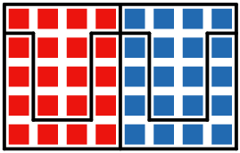
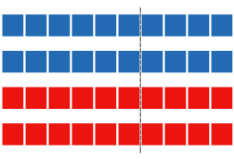
Red won 50% of the vote and 2 seats
Blue won 50% of the vote and 2 seats

Gerrymandered?

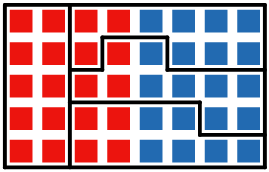
Red won 50% of the vote and 1 seat
Blue won 50% of the vote and 3 seats

How do we quantify gerrymandering?

Political gerrymandering’s opponents have argued that the process provides an unfair advantage for one party over another, contributing both to political polarization and the ability for a minority voice to control policy while silencing the will of voters. This argument has been brought before the Supreme Court in the past, most recently in the Vieth v. Jubelirer case in 2004. In this case, the Court ruled (by a 5-4 vote margin) that partisan gerrymandering was NOT unconstitutional. However, in his consenting opinion, Justice Kennedy wrote that he was indeed troubled by extreme partisan gerrymandering, but didn’t quite know how to define it and didn't want the courts to dabble in determining which individual congressional maps do and do not cross a reasonable threshold. This explanation left the door open for the gerrymandering argument to return to the court, with the directive that if a plaintiff could bring him a clear workable standard that clearly defines extreme gerrymandering, he may vote that district lines in violation of such a standard are unconstitutional.


This issue has once again resurfaced in front of the Supreme Court, this time in the case of Gill v. Whiftford, which is evaluating the constitutionality of Wisconsin’s state congressional map drawn by a Republican-controlled state legislature in 2011. Oral arguments for this case were held in October 2017, with a decision expected in the first half of 2018. In this case, political scientists Nick Stephanopoulos and Eric McGhee presented a three-part standard to classify what constitutes ‘extreme political gerrymandering:’

1. Was the map drawn with discriminatory intent - was there motive to benefit one party over another?


2. Did a map produce a 'large and durable' discriminatory benefit for one party over another? (this analysis will explore only this aspect of the standard presented)


3. Was there any legitimate justification for a map's discriminatory effect other than gerrymandering, such as changes in the natural political geographic landscape?

To address the second point of this standard, these researches constructed a metric that centers around looking at how many votes each party 'wasted' in a specific election, which they call the efficiency gap:

The Efficiency Gap

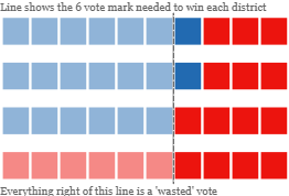
The efficiency gap measures the level of partisan bias in election results by quantifying foundational concepts to gerrymandering strategy, called ‘cracking’ and ‘packing’.

Cracking disperses opposting voters across a high number of districts where their candidates lose by narrow margins. Packing concentrates opposting voters into fewer districts where their candidates win by overwhelmingly high margins. Both of these strategies produce what political scientists call ‘wasted votes,’ which are votes that don’t directly contribute to the election of a candidate. So, all votes that are cast for a losing candidate or for the winning candidate above the 50% margin needed to win a district are considered ‘wasted’.

To efficiency gap metric first adds up all wasted votes for each party, then subtracts one party’s wasted votes from another. This difference is then divided by all votes cast to measuring the extent with which one party is more ‘cracked’ and ‘packed’ than the other party.

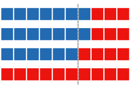
Let's look back at our example state and explore the district map that resulted in more districts won by the Blue party. How do we calculate the efficiency gap in this example? What was the efficiency gap in this example legislative map?

We can use these voting results in the efficiency gap formula to see how biased this election was, and which party it favored:

We first take the net wasted votes:

14 - 2 = 12



We then take these net wasted votes as a proportion of the overall votes cast:

12 / 40 = 15%



Finally, since this advantage favors the party who wasted less votes in the election, we find a:


15% efficiency gap benefitting Blue
in this example state.

Difference From Proportional Seats

While the constitutional right for proportional representation in legislatures does not exist, exploring the difference between the percent of votes won and districts won can give us a sense on how ‘fair’ election results were and what kind of congressional impact these results had on our lawmaking governmental wing. If one party won disproportionately more seats than they would have ‘expected’ to win based on their overall vote share, it might be worthwhile to examine this state's map in more detail.

In this analysis, the metric we'll call the 'difference from proportional seats' first determines how many districts one party would 'expect' to win in pure proportionality by multiplying the total districts available by the total percent of votes earned for that party. We then subtract the actual number of districts won by this party to find out how much over or under-representation this party enjoys in comparison to pure proportionality. Remember, each party in this example won 50% of the vote in a state with 4 seats up for grabs, so we'd 'expect' each party to win 2 seats if results were purely proportional:

Red won 1 of an expected 2 seats (-1)
Blue won 3 of an expected 2 seats (+1)


+1 net difference from proportional seat count benefitting Blue
in this example state.

Do these metrics show evidence of gerrymandering in the 2012 house elections?

If we implement these metrics with the real data from the 2012 elections, what do we find? The below analysis charts the results of the 2012 federal congressional elections, in which Republicans won a 33-seat advantage while losing the plurality of votes. Prior to these elections, Republicans gained control of many state legislatures, thus controlling redistricting processes that occured between the 2010 census and these congressional elections. We only look at states with more than two districts and use both the efficiency gap and difference from proportional seats to see if there is evidence of significant political bias in these elections at the state and district level. Explore the visualizations below to analyze the results and see if you think there's evidence of malicious gerrymandering influencing our federal House of Representatives.


NOTE: Plaintiffs in the ongoing Gill v. Whiftford Supreme Court case argue that a congressional districting map should only be illegal if the bias in the map drawing is deliberate, and not a factor of natural political geography. The below analysis only explores whether there is bias in the maps that were in use during the 2012 Congressional elections, NOT whether district lines should be conclusively considered unlawful if the Supreme Court rules in favor of the plaintiffs in this case. Further analysis would be necessary in states that display potential bias to determine if these results were deliberately constructed by parties in control of state legislatures at the time of redistricting, or whether they could have occurred naturally. Experts who have crafted the studies that explore this metric suggest a reasonable cut-off of an 8% efficiency gap, with anything above this line being considered unfairly biased. For reference, we’ve added this benchmark in the efficiency gap chart below to compare which states we might need to explore further.

State Results